II. EDA of BSSeq data generated from non-model organism in different conditions

BSXplorer allows for the categorization of regions based on their methylation level and density. This is done by assuming that cytosine methylation levels follow a binomial distribution, as explained in Takuno and Gaut’s research (please refer to [1, 2] https://doi.org/10.1073/pnas.1215380110 for details). The genes are then divided into three categories, BM (body-methylated), IM (intermediately-methylated) and UM (under-methylated), based on their methylation levels in the CG context using the following formula.

\[ CG<P_{CG};\ \ CHG/CHH>1-P_{CG} \]

\[ P_{CG}\le CG<1-P_{CG};\ \ CHG/CHH>1-P_{CG} \]

\[ CG/CHG/CHH>1-P_{CG} \]

The same rationale may be applied to other methylation contexts, as BSXplorer can produce \(P_{CHG}\) and \(P_{CHH}\) for CHG sites and CHH sites, respectively.

[1] Takuno S, Gaut BS. Body-Methylated Genes in Arabidopsis thaliana Are Functionally Important and Evolve Slowly. Mol Biol Evol. 2012;29:219–27.

[2] Takuno S, Gaut BS. Gene body methylation is conserved between plant orthologs and is of evolutionary consequence. Proc Natl Acad Sci. 2013;110:1797–802.

Categorisation with console script

Firstly, we will demonstrate the categorization of regions and their visualization using a console script.

bsxplorer-category -o TE_Cat_Report --dir TE_Cat -u 50 -d 50 -b 100 -S 10 --ticks \\-500bp \\ Body \\ \\+500bp -C 0 -V 50 -H 50 -q .75 --save_cat te_conf.tsv

A user can obtain a complete list of parameters by using the command bsxplorer-category –help. The configuration file has the following structure

Header should NOT be included in real config file.

sample group	Path to report	Path to genome	Flank length	Minimal length	Region_type
Misugi_mock	DRR336466.CX_report.txt.gz	TE.gff	500	0	match
Misugi_mock	DRR336467.CX_report.txt.gz	TE.gff	500	0	match
Misugi_infected	DRR336468.CX_report.txt.gz	TE.gff	500	0	match
Misugi_infected	DRR336469.CX_report.txt.gz	TE.gff	500	0	match

The bsxplorer-category command imports Bismark’s cytosine report file and performs a binomial test to determine the statistical significance of methylation at each site. The command uses the estimated error rate to conduct the test and generates corresponding p-values, which can be exported using the API. Additionally, the tool imports genomic annotation for each region in every context and calculates the PCG (or \(P_{CHG}\) or \(P_{CHH}\)) value. Finally, it filters and classifies the regions into UM, BM and other classes based on the results obtained.

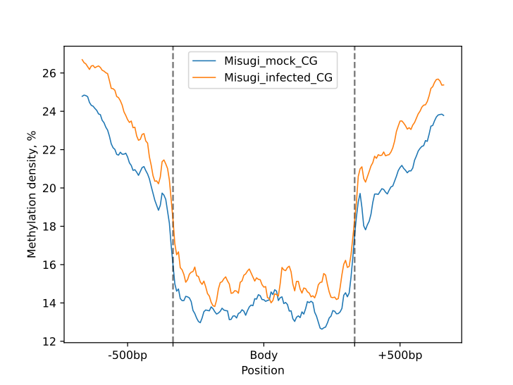
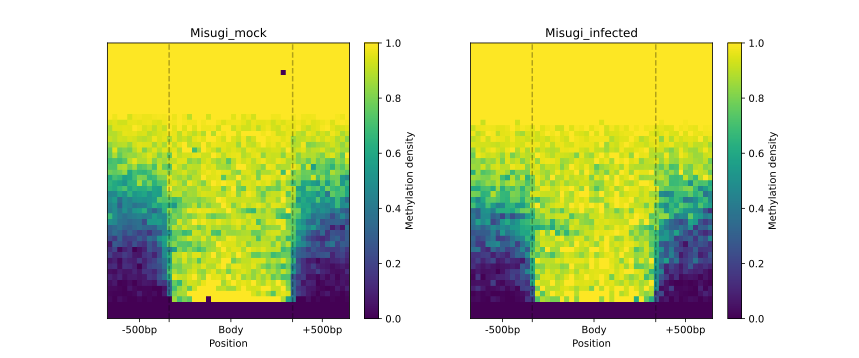
The following plots were generated for the BM and UM regions (CG-context) as part of the HTML-report.

Categorisation with Python API

The API version of the above command string is presented in the code snippet below:

annot = bsxplorer.Genome.from_gff("TE.gff")
annot = annot.other(region_type="match", flank_length=500, min_length=200)

mock_merged = merge_replicates(
    ["DRR336466.CX_report.txt.gz", "DRR336467.CX_report.txt.gz"],
    report_type="bismark"
)
inf_merged = merge_replicates(
    ["DRR336468.CX_report.txt.gz", "DRR336469.CX_report.txt.gz"],
    report_type="bismark"
)

p_value_kwargs = dict(
    genome=annot,
    methylation_pvalue=.05
)

mock_binom = bsxplorer.BinomialData.from_report(
    mock_merged.name, report_type="parquet", min_coverage=2
)
mock_pstat = mock_binom.region_pvalue(**p_value_kwargs)

inf_binom = bsxplorer.BinomialData.from_report(
    inf_merged.name, report_type="parquet", min_coverage=2
)
inf_pstat = inf_binom.region_pvalue(**p_value_kwargs)

categorise_kwargs = dict(
    context="CG", p_value=.05, min_n=5
)

# Returns tuple with (BM, IM, UM) ids
mock_cat = mock_pstat.categorise(**categorise_kwargs, save="mock")
inf_cat = inf_pstat.categorise(**categorise_kwargs, save="mock")

metagene_kwargs = dict(
    genome=annot,
    up_windows=50, body_windows=100, down_windows=50,
)
mock_metagene = bsxplorer.Metagene.from_binom(mock_binom.path, **metagene_kwargs)
inf_metagene = bsxplorer.Metagene.from_binom(inf_binom.path, **metagene_kwargs)

# e.g. for CG BM
metagenes = bsxplorer.MetageneFiles([
    mock_metagene.filter(context="CG", genome=mock_cat[0]), inf_metagene.filter(context="CG", genome=mock_cat[0])
], ["Mock", "Infected"])

tick_kwargs = dict(
    major_labels=["", ""],
    minor_labels=["-500bp", "Body", "+500bp"]
)

metagenes.line_plot(smooth=10).draw_mpl(**tick_kwargs)
metagenes.heat_map(50, 50).draw_mpl(**tick_kwargs)

For detailed explanation of used methods and parameters see:

• Basic usage tutorial

• bsxplorer.BinomialData

• bsxplorer.RegionStat

Conditions comparison

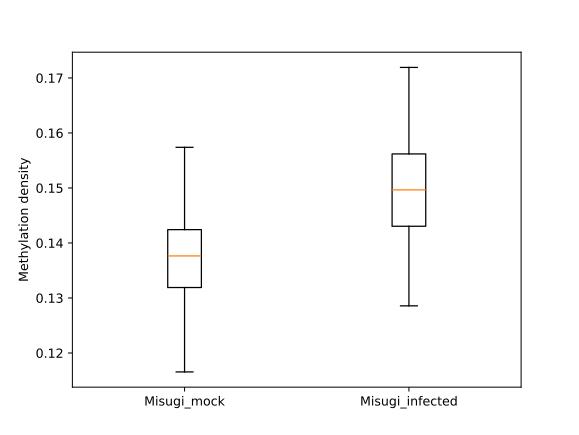
Using BSXplorer, the following section displays a practical approach to presenting these elements. The control and infected samples are referred to as “mock” and “inf” respectively. Here we assume that \(P_{CG}\) statistics which enables UM and BM classification has been computed in the previous steps of analyses (by --save_cat option of bsxplorer-category or save parameter of RegionStat.categorise()).

After importing the bisulfite data for the transposons (Misugi_mockCG_UM.tsv and Misugi_infectedCG_BM.tsv), the sets are intersected, matched with the annotation file, and the resulting patterns are visualized and compared to other regions.

Here we will use Polars (https://pola.rs/) module for DataFrames manipulation.

import polars as pl

# Read mock_UM and inf_BM TE IDs
mock_um = pl.read_csv("Misugi_mockCG_UM.tsv", separator="\t", has_header=False)[:, 3].to_list()
inf_bm = pl.read_csv("Misugi_infectedCG_BM.tsv", separator="\t", has_header=False)[:, 3].to_list()

# Intersect TE IDs from two groups
mock_inf_up = list(set.intersection(set(mock_um), set(inf_bm)))

# Load annotation file
te = bsxplorer.Genome.from_gff("TE.gff").other("match", 0, flank_length=500)

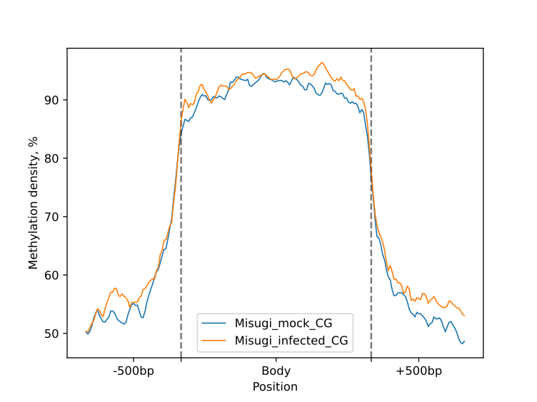
The metagenes are constructed using the mean statistics with the sumfunc="mean" parameter.

args = dict(genome=te, up_windows=50, body_windows=100, down_windows=50, sumfunc="mean")

# Read replicates metagenes
metagene_mock = bsxplorer.MetageneFiles.from_list(["DRR336466.CX_report.txt.gz", "DRR336467.CX_report.txt.gz"], labels=["mock-1", "mock-2"], **args)
metagene_inf = bsxplorer.MetageneFiles.from_list(["DRR336468.CX_report.txt.gz", "DRR336469.CX_report.txt.gz"], labels=["inf-1", "inf-2"], **args)

# Merge biological replicates
metagene_mock = metagene_mock.merge()
metagene_inf = metagene_inf.merge()

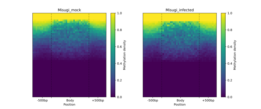
The .merge() method of the MetageneFiles class is used to combine biological replicates. The following code snippet creates a clustergram for a selected subset of genomic regions of interest using the .dendrogram() function.

# Construct a MetageneFiles object to visualize dendrogram
dendro_metagene = bsxplorer.MetageneFiles([metagene_mock.filter(id=mock_inf_up), metagene_inf.filter(id=mock_inf_up)], ["mock_up", "inf_up"])

dendro_metagene.dendrogram(q=0)

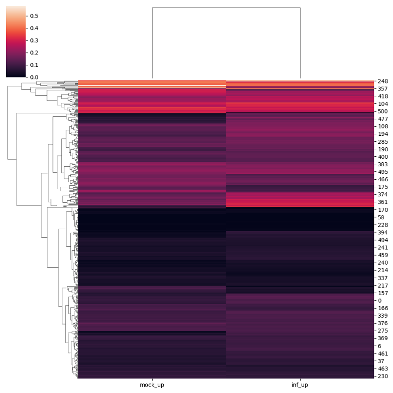
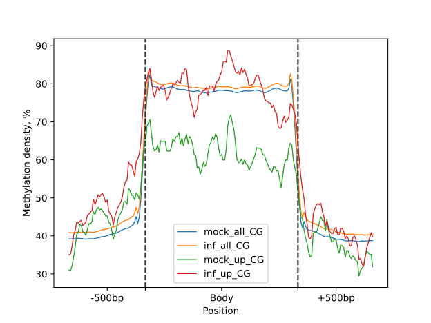
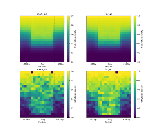
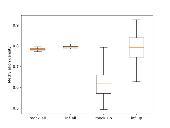
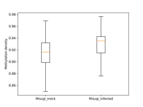
To visually compare the UM and BM regions that contain transposable elements with the remaining genomic regions that exhibit UM or BM patterns, we create a MetageneFiles object. This object enables us to generate line and box plots, as well as heatmaps that display methylation levels in the aforementioned classes.

metagenes = bsxplorer.MetageneFiles(
    [metagene_mock, metagene_inf, metagene_mock.filter(id=mock_inf_up), metagene_inf.filter(id=mock_inf_up)],
    ["mock_all", "inf_all", "mock_up", "inf_up"]
)
filtered = metagenes.filter(context="CG")

ticks = {"major_labels": ["", ""], "minor_labels": ["-500bp", "Body", "+500bp"]}
filtered.line_plot(smooth=10).draw_mpl(**ticks)
filtered.heat_map(20, 20).draw_mpl(**ticks)
filtered.trim_flank().box_plot().draw_plotly()