Getting started

This page will give you the overview of the BSXplorer analysis scenarios.

• Basic usage

• Clustering of methylation patterns

Basic Usage

The analysis process can be divided into four steps as follows:

1. Import annotation file

2. Read Bismark’s cytosine report file

3. Get results

The example analysis is prepared for Arabidopsis thaliana chromosome 3 (NC_003074.8). The test data can be downloaded from the Zenodo repository.

Import annotation file

Firstly we need to import bsxplorer module.

import bsxplorer

To import genome annotation from file use BSXplorer function bsxplorer.Genome.from_gff(). The parameters provided to the function include a path to the annotation file in GFF format.

genome = bsxplorer.Genome.from_gff("arath_genome.gff")

Next, the annotation is filtered to extract the genomic regions of interest. E.g. this can be achieved with gene_body() function from the class Genome, to filter only genes from annotation.

genes = genome.gene_body(flank_length=2000, min_length=3000)

Upon completion of these steps, the annotation file can be combined with the methylation data from the cytosine report, making it possible to perform analyses of DNA methylation patterns within particular genomic contexts.

Read report

To analyse the cytosine report and carry out metagene analysis, BSXplorer offers the Metagene class. In order to read the Bismark’ methylation_extractor output file, the function from_bismark() of the Metagene class should be utilised.

metagene = bsxplorer.Metagene.from_bismark("arath_example.txt", genes, up_windows=100, body_windows=200, down_windows=100)

Get results

Depending on the analyses goals it may be required to filter the cytosine report file to extract information on the methylation context of interest as well as on strand attribution of a methylation event. This is achieved by using the Metagene.filter() function:

filtered = metagene.filter(context="CG", strand="+")

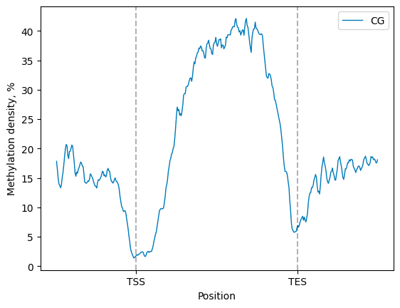
The smoothened matplotlib line plot, showing the average methylation density in the metaregion of interest (e.g., gene body, plus upstream and downstream regions of desired length), can be generated with the Metagene.line_plot().draw_mpl()

filtered.line_plot(smooth=10).draw_mpl()

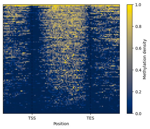
Alternatively, a heatmap representation of the methylation signal density is made available by application of the Metagene.heat_map().draw_mpl() method.

Clustering of methylation patterns

BSXplorer allows for discovery of gene modules characterised with similar methylation patterns.

arath_genome = bsxplorer.Genome.from_gff("arath_genome.gff")
arath_genes = arath_genome.gene_body(min_length=0, flank_length=2000)

arath_metagene = bsxplorer.Metagene.from_bismark(
    "arath_example.txt", arath_genes,
    up_windows=5, body_windows=10, down_windows=5
)

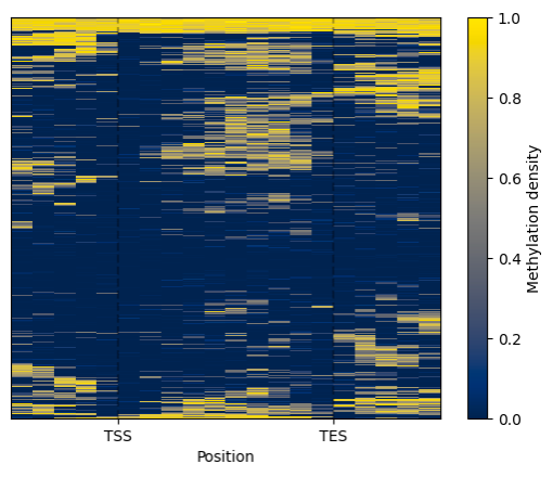
Once the data was filtered based on methylation context and strand, one can use the .cluster() method. The resulting ClusterSingle object contains an ordered list of clustered genes and their visualisation in a form of a heatmap.

arath_filtered = arath_metagene.filter(context="CG", strand="+")
arath_clustered = arath_filtered.cluster(count_threshold=5, na_rm=0).all()

To visualise the clustered genes, use the .draw_mpl() method.

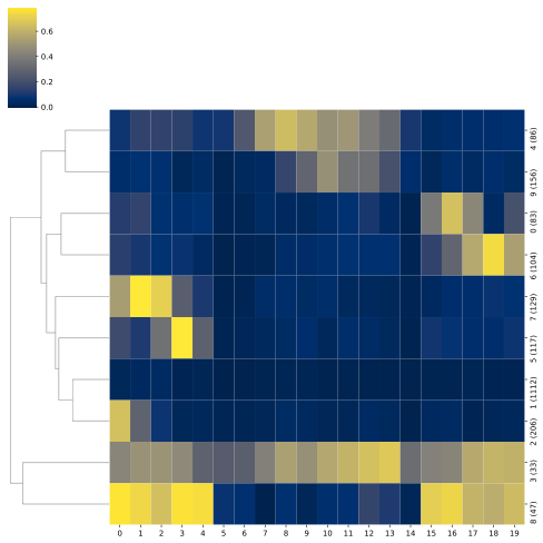
To identify gene modules that exhibit similar methylation patterns apply the .modules() function of the Clustering class. This method relies on the dynamicTreeCut algorithm to find modules.

arath_modules = arath_filtered.cluster(count_threshold=5, na_rm=0).kmeans(n_clusters=5)
arath_modules.draw_mpl()